Applying Machine Learning

In the autumn of 2022, thousands of berry images were stored among the large image metadata, the machine learning model was finalized and the final project seminar was kept. Berry machine -project ended and it was a fascinating journey into practical machine learning.

The Berry machine project was financed by Interreg Nord with Natural Resources Institute Finland (LUKE) and the Norwegian Institute of Bioeconomy Research (NIBIO) participating, Frostbit Software Lab at Lapland University of Applied Sciences as a developer. The project goal was to study the possibility to use machine learning to make the current berry harvest estimation measurement process less dependent on manual labour, thus bringing up the possibility to do significantly more field measurements and open up new ways to estimate berry yields.

Current berry harvest estimation measurement is done by manually counting every single berry inside a frame created with various materials (Kilpeläinen 2016). The frame forms precisely one m² area. In the forest, five frames are installed in places with varying ground types (marjahavainnot.fi 2022). After all of this manual work, data is still not exhaustive enough to do more elaborated studies as the process is both expensive and laborious (Bohlin 2021).

The Berry machine project studied the way how to use deep learning to help count the berries and thus make the process significantly less laborious. The plan was to use deep-learning computer vision to detect berries and create a functioning prototype system with a mobile application and all required backend applications.  Only bilberry (Vaccinium Myrtillus) was required as the initial target species, but lingonberry (Vaccinium Vitis-idea) was also included to give a more comprehensive view of how the berry machine system would work across species. Both of the berries were counted in growth phases “flower”, “raw” and “ripe”.

The main steps to fulfill the Berry machine project task were to train a computer deep learning model to detect berries from images. Using this computer vision, berries were counted from images and the detected berries count was compared to the number of berries counted by field measurement.

Traditional Artificial Neural Network (ANN) is formed with input neurons, hidden layers and an output layer (Figure 1). In the case of image classification, input image pixel values are added as values in the input layer (Gogul 2017). Weight and bias values in hidden layer neurons and connections are derived in the training process. Weight and bias are then used to recalculate new values for input values when all original pixel values propagate from left to right arriving finally at the final output layer representing the result in numerical form.

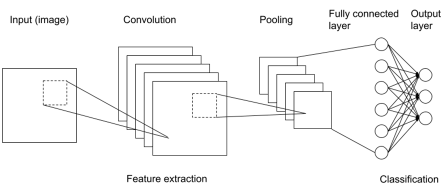
Compared to the ANN, image classification results are significantly improved changing to breakthrough technology, Convolutional Neural Network (CNN) (Marmanis 2016). CNN architecture improves ANN architecture by adding convolution and pooling layers. New layers simplify and extract features of the image while keeping the feature position with the original image (Figure 2). Pooling layers sub-sample the original image and feature extraction layers detect more high-order features from the image. With CNN architecture, computer vision is capable of human-level or higher accuracy (Galanty 2021).

CNN architecture on its own only classifies one image as a whole. The project goal with computer vision was to detect multiple instances of berries in various growth phases from a single image. Therefore object detection architecture is required instead of image classification architecture as object detection also seeks to locate berry instances from their natural background (Liu 2018).

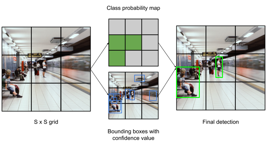
Object detection architecture YOLO (You Only Look Once) was used in the project. YOLO was designed to be fast, simple and accurate (Redmon 2015). The YOLO process splits the image into a grid and detects objects in each grid and predicts the bounding boxes. Bounding box results are joined with the classification probability of each grid to filter more accurate results (Redmon 2015).  The YOLO process is visualized in Figure 3. YOLO version 5 was used in the project as it was built using PyTorch framework (Solawetz 2020) which did make it easier to implement. As a bonus, YOLOv5 added data augmentation to the training process out of the box (Benjumea 2021).

A deep-learning training dataset was formed by taking thousands of berry images. Approximately 10 000 images were collected using mostly consumer-level mobile phones. One of the ideas in the original project plan was to get closer to crowdsourcing the berry harvest measurements with an ease-of-use mobile application. Therefore training was to be done mostly using phones available to the general public.

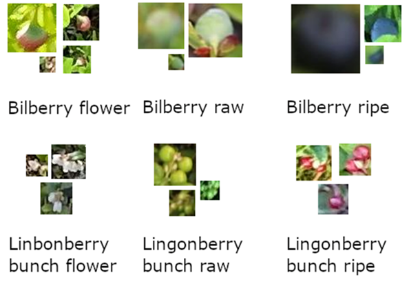
After and during the dataset collection, the annotation process was initiated. The annotation process was very labour-intensive and not all images were annotated due to limits in resources. The annotation process is simply manually drawing the correct berry class on top of the image. A significant difficulty was that berries are small and especially raw berries hide well in the background. After the main dataset of annotated images was complete, additional annotation processes were initiated to balance the dataset. The balance dataset is a training dataset with a roughly equal number of instances from each class. The final dataset was formed of six classes shown with examples in Figure 4.

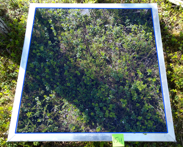
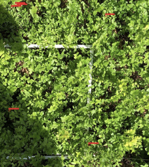
The density formula is the number of instances divided by area. Computer vision was used to estimate the number of berries but the surface area was missing. The field measurement counting frames were also annotated for density estimation as in Figure 5. Frame polygon was used to crop deep learning detected berries and thus all berries left in the image were inside from a one m² and 0,25 m² area. Two different sizes of count frames were used to allow comparing detection correlation differences in images taken closer and further off the ground.

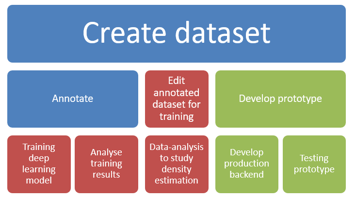
The Berry machine tasks were visualised in Figure 6. A significant amount of work was used to analyse and improve iteratively training results. Improving training results meant that more annotation was done as sometimes data was not balanced enough. The computer was not the only one with difficulties detecting berries as annotating was also difficult due to a larger number of obscure berries barely visible in images. It is likely that if personnel was directed to annotate the same images, results would vary.

The main dataset processing before the training was the process of splitting the image into smaller pieces. The YOLOv5 model used in the project had a native resolution of 640×640 pixels. Inputting a larger image meant downscaling into the native resolution. As images were taken with, for example, 4032×3024 resolution, significant loss of detail would occur which is detrimental when detecting small instances like berries. Therefore all annotated images annotated in their original resolution and all images from where berries were detected, would be split into smaller images before detection and training. A complex splitting algorithm with overlapping zoom levels was initially used, but the splitting process was reverted to a more simple split process as simpler process advantages were more numerous than using more complex methods. Once again, simplicity wins.

Training iterations were not exhaustively laborious by themselves, but with deep learning, improvements were done by modifying the dataset and the dataset pre-processing which was time-consuming. Project time was also used in post-process as training results required analysis and detection quality checks in some cases using a benchmark dataset.

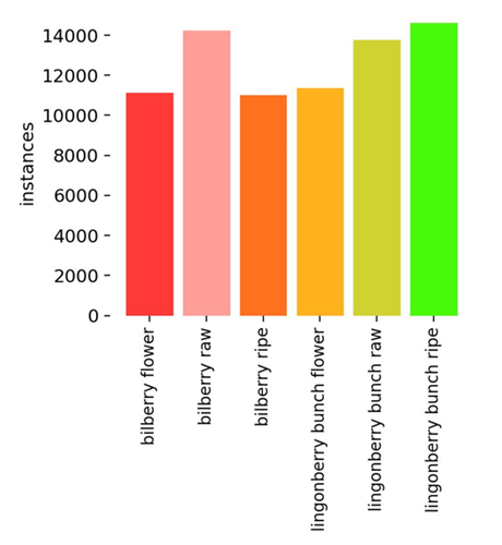
The final training dataset of image pieces normalized to 640×640 pixels used for training was 41 101 images with 95 065 annotated berries. Dataset was supplemented with synthetic data created randomly adding clipped berry images with transparent backgrounds on top of various background images. Background images were mostly images taken around the campus and plain white background images. Figure 7 visualizes the final balance of the dataset. Balance was deemed sufficient based on the graph.

As presented in Figure 8, the project’s backend architecture was made into four separate services. The prototype backend was the main backend for the prototype mobile application. The prototype backend’s main tasks were to add login property, act as image storage for images uploaded and store location and result values. The dataset inference process service’s purpose was to batch-run the detection process to thousands of images and save results for data analysis. The resulting metadata of detected berries was used for the density estimation study. The pipeline backend’s main task was to split the image and request detection backend for each split image. After all the image slices were executed through the detection backend, the detected berries’ position in the image slice was converted to the original main image. Finally, all results were sent to the address defined in the original request. The final backend was the inference backend which ran the model detection with the image received and responded with the detection results.

Prototype application development was initiated after the first viable detection model was trained. The main architectural decision with the prototype application backend was to build the actual deep learning backend (inference backend) into a separate service. The decision was made to allow separate backend deployment on various Graphical Processing Unit (GPU) or non-GPU servers. In addition, the image split backend was developed into a separate service to minimally modify the standard prototype backend used by the prototype application. This was to make it easiest to deploy the prototype backend using an existing headless API and allow using the image split-enabled detection backend (pipeline backend) past the prototype backend presented in Figure 8. Modular design as architectural design separates concerns more reliably, but in practice, it was noted, that deployment of multiple services on each edit slowed the process significantly and thus increased complexity.

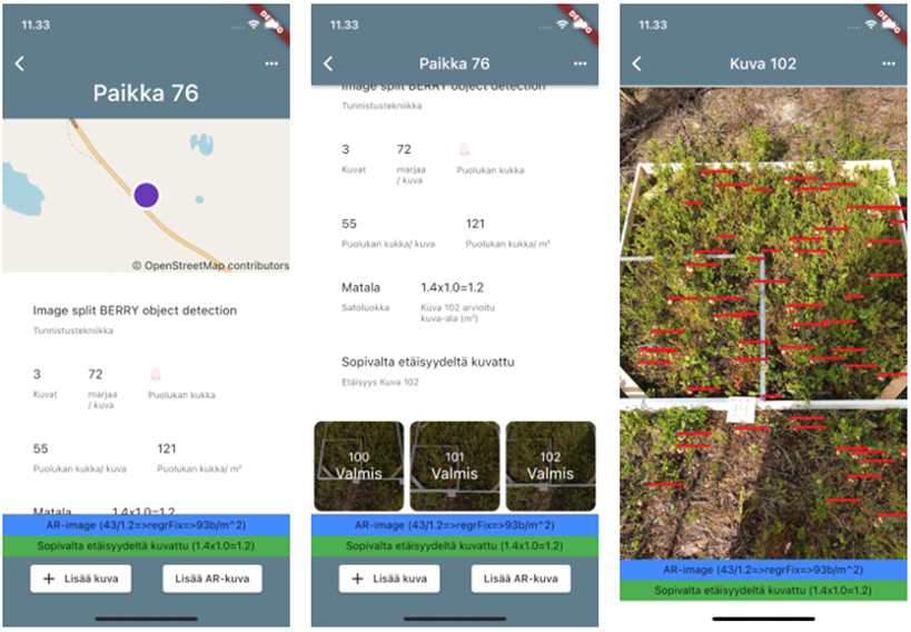
The prototype application was developed using a multiplatform Flutter framework that enables developing for both IOS, web and Android using the same codebase (GitHub.com 2022). On measurement location, the user created a new location from the UI. The location user interface is visualized in Figure 9. The location page showed the estimated berry density among other information. The target berry phase and species were defined by the most prominent berry detected from multiple images. Density was estimated as the average of all images and corrected with a linear regression formula derived from the correlation analysis. Surface area estimation for density calculation was tested with two different methods. First, estimate the area from the berry average size. The second method was to estimate the area using augmented reality (AR) libraries. AR was implemented only in Apple IOS devices.

In the project, multiple different results emerged: Deep learning detection model results and density estimation results. Detection results are covered first. The results are from the last training iteration.

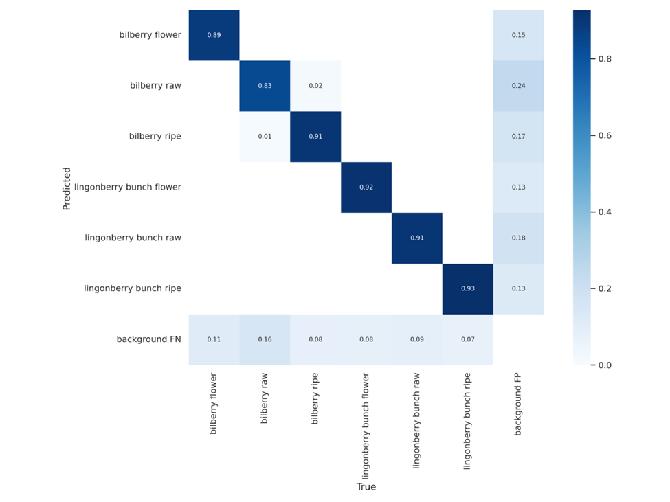
In the YOLOv5 deep learning process dataset of annotated image pieces was split into three parts. Training test and validation. The training dataset was used to train the model, the test dataset was used to test the model’s progress during training and the validation dataset was to do final testing after the training was done. Validation dataset results indicated a detection rate from 83% to 93% depending on the class. Results are visualized with the confusion matrix in Figure 10. The confusion matrix depicts percentages of predicted detections matching the true values. Reading the confusion matrix in the case of class bilberry ripe detections, 1% was bilberry raw, 91% correct and 17% of the ripe bilberries detected were part of the background. According to the confusion matrix, ripe lingonberries were the most detected class while bilberry raw had significantly worst results. Overall, the results were deemed acceptable.

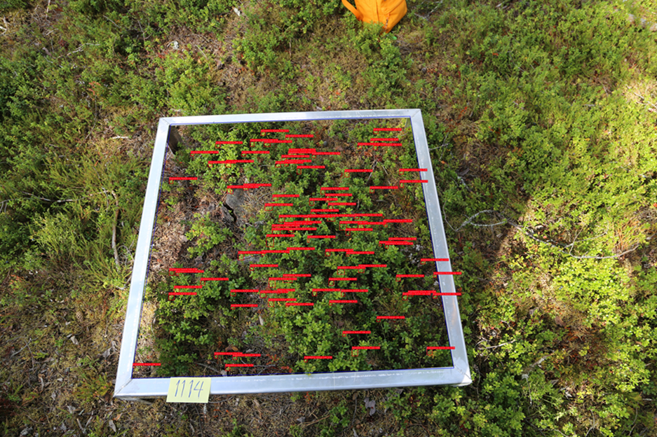
For the density estimation study, the trained model was executed to detect berries in nearly 5000 images with one m² and 0,25 m² frame annotations. Frame annotation was then used to crop detected berries and only inner berries were kept (Figure 11).

estimated density = (number of detected berries of the correct type) / (frame surface area)

Equation 1. Calculate the estimated berry density

For density calculation, the surface area was defined by frame area and the number of berries was the cropped value of deep learning detected berries of the same type as calculated in the image. Every image file path defined the target berry species, growth phase and location. This meta-information was used to filter only target classes into density estimation. Density estimation was calculated for each image with Equation 1.

The estimated density was not the final result used in the prototype. The assumption was that image will not show all berries present, but berry detection in the image correlates with the field measurements. Linear regression formula was derived using the correlation. For each class, the regression formula in the prototype was different.

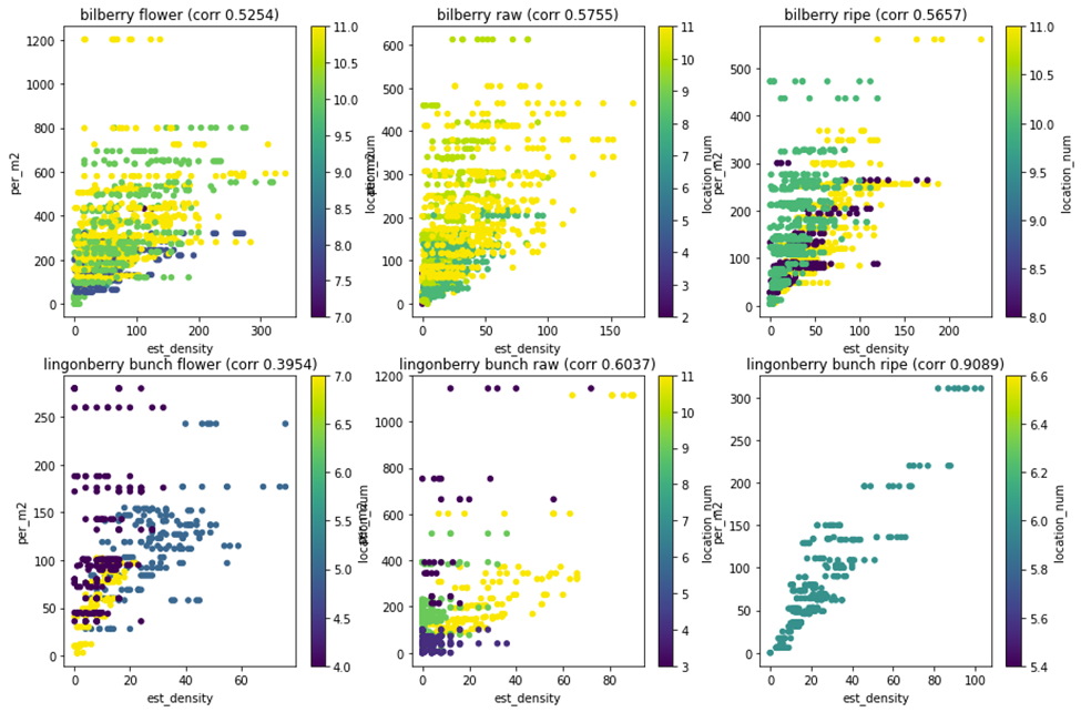
Estimated density and field measurement value was plotted into scatter plot for each class separately (Figure 12). Pearson correlation for each class was shown in the scatter plot in the plot title. The Scatter plot was coloured by location to visualize how location affects the relation between detected berries and the field berry count. The Scatter plot shows several points:

• Ripe lingonberry has fewer data and all of the ripe lingonberry images are only from 2021 images. More homogenous ripe lingonberry data hints at the need for more varied data as homogenous datasets can lead to early conclusions.
• To practically use correlation with for example linear regression to estimate density from the image, more variables need to be taken into consideration. Location colouring hints at one additional way to improve correlation by considering growth location.
• Bilberry and lingonberry behaviour were different. With bilberry, possible causes of noise can be more lush undergrowth than lingonberry blocking camera view of the berries.
• Lingonberry was detected as bunches, but field measurement calculated lingonberries as individual berries. The difference between berry count and bunch count is likely to increase with increased yield. Lingonberry may grow more berries in a single bunch when the berry harvest improves.

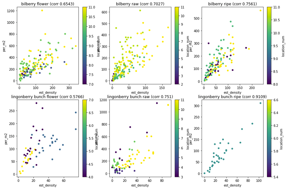
One method of increasing correlation results was to take all the images taken from the same frame and use only the image with the most berries detected. In theory, only the image with the best angle and quality to capture most berries is used. This required taking multiple images from a single frame. Practical challenges in image quality were sun position with the camera causing difficulty to detect individual berries, camera shake and angle with more ground vegetation in the way. Using the image with the most berries was justifiable and the maximum value image did give a better correlation than the average value. With the maximum value image, correlation with the field measurement value was improved (Figure 13).

Detecting berries in different growth phases using consumer-level cameras and deep-learning object detection yielded successful results. Computer vision with object detection is a highly viable method of detecting difficult instances from the natural background. Invaluable information about practical machine learning processes especially concerning data pre- and post-processing was collected. In the project, large and valuable training data was created from the field measurements to the additional synthetic dataset.

Density estimation was as not simple as many things in nature are. A perfect example of the challenges was shown in Figure 14 with bilberry. High-yield bilberry harvest is accompanied by lush ground vegetation. This inversely lowers the number of detected berries in the image.

The project gave a more in-depth view of the ways to estimate density and how to approach the problem. The main challenges with the density estimation were berry detection, surface area estimation and density estimation with the information collected. Berry detection was deemed feasible, but the other two require more studies.

Surface area estimation was tested in the prototype with two different methods. Using detected berries as a base measurement to estimate image cover area and using the operating system’s augmented reality (AR) framework. AR was deemed the preferable method in the long term. The project prototype proved that AR can be used to measure ground area, but requires a significant amount of software development to be viable. Challenges include detecting flat plane on a practically uneven surface and handling noise in AR measurement caused by constantly moving cameras and implementing AR on both of the most common phone operating systems.

Concerning density estimation with surface area and berry detection results, more research is required. Correlation does exist but is too weak to be practical. Directing users to take multiple images and using images with the most berries detected, is one viable option to improve the correlation, but more data dimensions are needed. Berry’s growth location shows promise as one dimension to factor in.

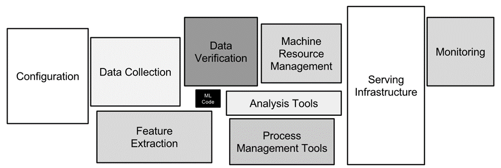
With the deep-learning process, a considerable amount of experience was collected. Practical experiences in the project correlated with the argument expressed in the article “Hidden Technical Debt in Machine Learning Systems” that Machine Learning (ML) systems have a special capacity for causing technical dept (Sculley 2015).  The article also states that only a tiny fraction of the code in an ML system is for the actual training or prediction (Figure 15). Berry machine project code base supported this statement. A large amount of code was required to modify and create a dataset in the post-process. ML backend deployment with modular design, version verification and generic request and response formats also increased the codebase a significant amount. The final part often overlooked was the analysis process tools to draw conclusions and guide the iterative training process in the correct direction.

As stated by Sculley 2015, Using generic packages in a hope that it reduces the amount of coding required, often results into glue code to join generic packages together. The glue code issue led to the project developing custom packages for project purposes. Version control was one difficult aspect, as the ML system was improved by modifying the large training dataset not managed by a version control system. Thus it is difficult to duplicate results in a specific version without the correct training dataset.

Implementing a real-world ML system can be a hassle. A large number of surrounding infrastructure is required in the system. Infrastructure is not inherently negative, but a valuable lesson is to consider this requirement when creating an ML system. When implementing an ML system, obstacles differ from a normal software project. Before and during the process, developers need to be careful not to end up filling the system with anti-patterns like glue-code, pipeline jungles and abstraction dept (Sculley 2015).

In the end, the Berry machine project was a priceless experience filled with hope and excitement. The project generated numerous internships and launched two bachelor’s theses and one master’s thesis. Practical ML system experience was learned. Hopefully, we will see more ML usage in the future as the potential is tangible.

Benjumea, Aduen, Izzedin Teeti, Fabio Cuzzolin, and Andrew Bradley. YOLO-Z: Improving small object detection in YOLOv5 for autonomous vehicles. arXiv preprint arXiv:2112.11798, 2021.

Bohlin, Inka. Maltamo, Matti. Hedenås, Henrik. Lämås, Tomas. Dahlgren, Jonas. Mehtätalo, Lauri. ”Predicting bilberry and cowberry yields using airborne laser scanning and other auxiliary data combined with National Forest Inventory field plot data.” Forest Ecology and Management, Volume 502. ISSN 0378-1127, 2021.

Galanty, Agnieszka . Tomasz Danel, Michał We˛grzyn, Irma Podolak. ”Deep convolutional neural network for preliminary in-field classification of lichen species.” 2021.

GitHub.com. Flutter SDK. 2022. https://github.com/flutter/flutter (retrieved 7. 12 2022).

Gogul, I. and Kumar, Sathiesh. ”Flower species recognition system using convolution neural networks and transfer learning.” 2017.

Kilpeläinen, Harri. Miina, Jari. Store, Ron. Salo, Kauko Salo. Kurttila, Mikko. ”Evaluation of bilberry and cowberry yield models by comparing model predictions with field measurements from North Karelia, Finland.” Forest Ecology and Management, Volume 363. ISSN 0378-1127, 2016. 120-129.

Liu, Li & Ouyang, Wanli. Wang, Xiaogang. Fieguth, Paul. Chen, Jie. Liu, Xinwang. Pietikäinen, Matti. ”Deep Learning for Generic Object Detection: A Survey.” International Journal of Computer Vision. 2018.

marjahavainnot.fi. ”Luonnonmarjojen satohavainnot.” 2022. https://marjahavainnot.fi/assets/info/Havaintometsan_perustaminen_v2.pdf (retrieved 25. 4 2022).

Marmanis, Dimitris and Wegner, Jermaine and Galliani, Silvano and Schindler, Konrad and Datcu, Mihai and Stilla, Uwe. ”SEMANTIC SEGMENTATION OF AERIAL IMAGES WITH AN ENSEMBLE OF CNNS.” ISPRS Annals of Photogrammetry, Remote Sensing and Spatial Information Sciences. 2016. 473-480.

Redmon, Joseph. Divvala, Santosh Kumar. Girshick, Ross B. Farhadi, Ali. ”You Only Look Once: Unified, Real-Time Object Detection.” CoRR abs/1506.02640. 2015.

Sculley, D. and Holt, Gary and Golovin, Daniel and Davydov, Eugene and Phillips, Todd and Ebner, Dietmar and Chaudhary, Vinay and Young, Michael and Crespo, Jean-François and Dennison, Dan. ”Hidden Technical Debt in Machine Learning Systems.” Advances in Neural Information Processing Systems. 2015.

Solawetz, Jacob. YOLOv5 New Version – Improvements And Evaluation. 29. 6 2020. https://blog.roboflow.com/yolov5-improvements-and-evaluation/ (retrieved 25. 4 2022).

This article has been evaluated by the FrostBit’s publishing committee, which includes Heikki Konttaniemi, Toni Westerlund, Jarkko Piippo, Tuomas Valtanen, Pertti Rauhala and Tuuli Nivala. The article publications can be found on the FrostBit publication blog.

—— 17.12.2022 ——

SHARE IN